Basics of Neural Network Programming
Binary Classification
바이너리(0 또는 1)로 분류하는 것을 의미한다.
예를 들어 고양이의 이미지를 보고 고양이인지(1) 아닌지(2)를 판단해 라벨을 다는 것은 binary classification이다.
Notation
$n_x$ features : $x$, output $y$
$x \in \reals^{n_x} , \ y \in {0,1}$
m개의 training example : ${(x^{(1)},y^{(1)}),(x^{(2)},y^{(2)}),...,(x^{(m)},y^{(m)})}$
$$X = \begin{bmatrix}
x^{(1)} \ x^{(2)} \ ... \ x^{(m)}
\end{bmatrix}
\
X \cdot shape = (n_x,m)$$
Feature Vector $X$는 $n_x \times m$ matrix이다.
다른 표기에서는 $X$를 transpose하여 만드는 경우도 있지만, 코드 작성의 편의를 위해 위와 같이 표기한다.
$$Y = \begin{bmatrix}
y^{(1)} \ y^{(2)} \ ... \ y^{(m)}
\end{bmatrix}
\
Y \cdot shape = (1,m)$$
Logistic Regression
$x$가 주어졌을 때, $\hat{y} = P(y=1|x)$ ($y=1$일 확률)을 구한다.
- 파라미터$b \in \reals$
- $w \in \reals^{n_x}$
- 출력
- $\hat{y} = \sigma(w^Tx+b)\ \ \ \ =\sigma(z)= \frac 1 {1 + e^{-z}}$

Logistic Regression cost function

Training set$(x^{(i)},y^{(i)})$이 주어졌을 때,
알고리즘의 $y=1$일 확률이 실제와 비슷해지기를 원한다. ($\hat{y}^{(i)} \approx y^{(i)}$)
- Loss (error) Function :오차 함수가 최대한 작게 만들기를 원한다.
- $-(y \log \hat{y} +(1-y)\log(1-\hat{y}))$

- Cost Function파라미터 $w, b$를 조절해서 cost function $J$가 최소가 되도록 하는 $w, b$를 찾는다.
- $$J(w,b) = \frac 1 m \sum^m_{i=1}[y^{(i)} \log \hat{y}^{(i)}+(1-y^{(i)})\log(1-\hat{y}^{(i)})]$$
Gradient Descent

이를 통해 cost function의 global optimum을 찾고 이때의 $w,b$를 구한다.
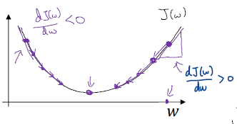
수렴할 때까지 다음 식을 반복한다.
$w := w - \alpha \frac {\partial J(w,b)} {\partial w}$
$b := b - \alpha \frac {\partial J(w,b)} {\partial b}$
Derivatives

More derivatives examples

Computation Graph
변수의 관계와 흐름을 파악할 수 있는 그래프이다.
오른쪽으로 가면 어떤 변수가 어디에 들어가는지, 왼쪽으로 가면 미분할 때 유용하게 사용할 수 있다.

Derivatives with a Computation Graph
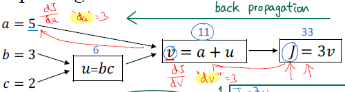
$u =bc, \ v=a+u, \ J=3v$ 일 때

- $J=3v$ 이므로$\therefore \frac {dJ} {dv} = 3$
- $v =11 \to 11.001$ 이 되면, $J=33 \to 33.003$ 이 된다.

- $v=a+u$ 이므로연쇄법칙 (chain rule)에 의해서,$\therefore \frac {dJ} {db} = \frac {dJ} {du} \cdot \frac {du} {db} = 3 \times c$
- $\therefore \frac {dJ} {dc} = \frac {dJ} {du} \cdot \frac {du} {dc} = 3 \times b$
- $\therefore \frac {dJ} {da} = \frac {dJ} {dv} \cdot \frac {dv} {da} = 3 \times 1$
- $a = 5 \to 5.001, \ v=11 \to 11.001, \ J=33 \to 33.003$
또한, 이 강의에서 $\frac {d[FindOutputVar]} {d[var]}=d[var]$ 로 약속하고 사용한다.
Logistic Regression - Gradient Descent
Logistic Regression recap
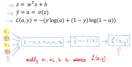
Logistic Regression derivatives

$$[da]=\frac {dL(a,y)} {da}=-\frac y a + \frac {1-y} {1-a}$$
$$[dz]=\frac {dL(a,y)} {dz}=a-y$$
Gradient descent on m examples
$$J(w,b)=\frac 1 m \sum^m_{i=1}L(a^{(i)},y^{(i)})
\
\to a^{(i)}=\hat{y}^{(i)}=\sigma(z^{(i)})=\sigma(w^Tx^{(i)}+b)$$
$$\frac \partial {\partial w_1}J(w,b)=\frac 1 m \sum^m_{i=1}\frac \partial {\partial w_1}L(a^{(i)},y^{(i)})$$
Initialize values : $J=0, \ dw_1=0, \ dw_2=0, \ db = 0$
For $i=1 \ to \ m$:
$z^{(i)}=w^Tx^{(i)}+b$
$a^{(i)}=\sigma(z^{(i)})$
$J \larr J + -[y^{(i)}\log a^{(i)} + (1-y^{(i)})\log (1-a^{(i)})]$
$dz^{(i)}=a^{(i)}-y^{(i)}$
$dw_1 \larr dw_1 + x_1^{(i)}dz^{(i)}$
$dw_2 \larr dw_2 + x_2^{(i)}dz^{(i)}$
$db\larr db + dz^{(i)}$
Compute Average:
$J/m, \ dw_1/m, \ dw_2/m, \ db/m$
$dw_1=\frac {\partial J} {\partial w_1}$
For
$w_1 :=w_1-\alpha dw_1$
$w_2 :=w_2-\alpha dw_2$
$b :=b-\alpha db$
for문이 이중으로 반복되기 때문에 비효율적이라는 단점이 있다.
이후 Vectorization을 통해 이를 해결할 수 있다.
Source
Neural Networks and Deep Learning
신경망 및 딥 러닝
deeplearning.ai에서 제공합니다. In the first course of the Deep Learning Specialization, you will study the foundational concept of neural networks and ... 무료로 등록하십시오.
www.coursera.org